
Most satellite vegetation monitoring measures greenness: where vegetation exists, its density, or whether it is becoming greener or browner over time. But many environmental and land-management decisions depend on something more structural: how tall vegetation is, how canopy structure changes over time, and where vegetation is being cleared, degraded, or recovering.
Geoneon developed a vegetation height monitoring workflow that estimates mean vegetation height at 10 metre resolution from Sentinel-2 imagery across the Pacific. Built as a quarterly time-series dataset spanning 2020–2025, the system enables consistent monitoring of vegetation structure change over time, supporting applications such as deforestation tracking, regrowth monitoring, restoration planning, biomass estimation, and climate reporting.
This work was delivered by Geoneon and D4DInsights in partnership with the Pacific Community (SPC) through its Digital Earth Pacific programme, which commissioned and guided the development to address regional priorities. The Digital Earth Pacific and D4DInsights contributors, included Andiswa Mlisa, Sachindra Singh, Aditya Agrawal, Brian Killough, Alex Leith, and Jesse Anderson.
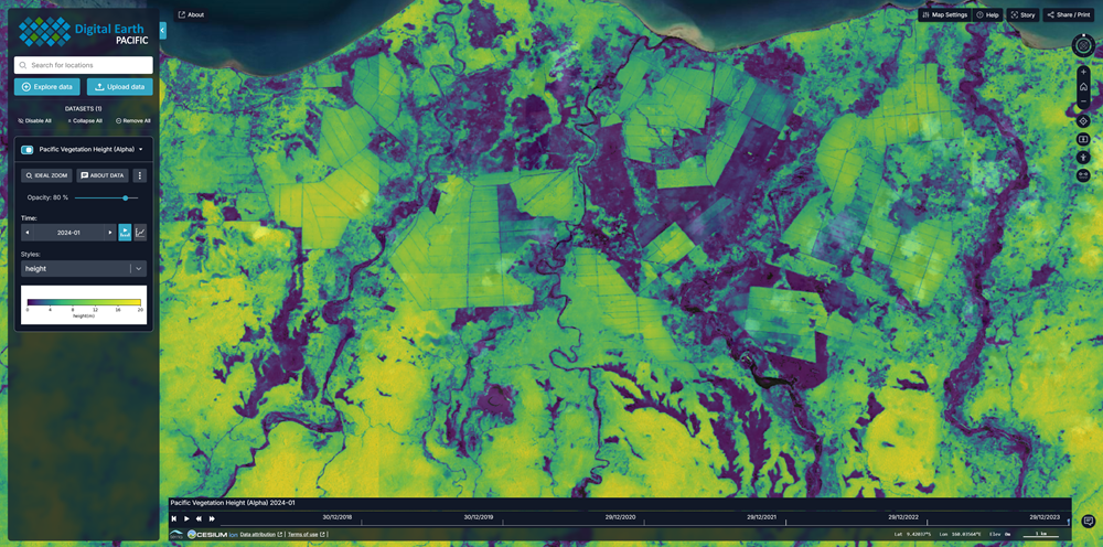
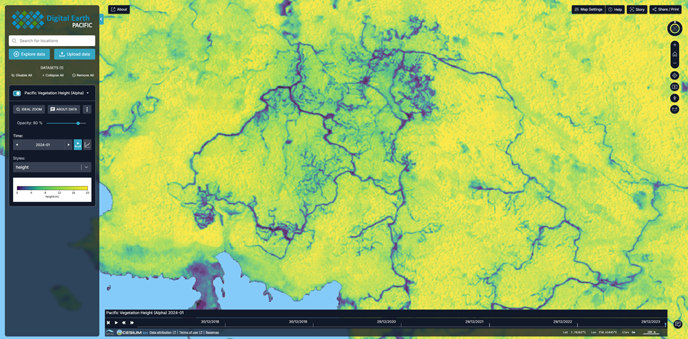
Fig. 1. The Digital Earth PACIFIC platform, showing vegetation structure changes across the Pacific between 2020 and 2025.
Executive Summary
Most satellite vegetation monitoring products focus on greenness or land cover. Geoneon’s workflow instead focuses on vegetation structure: estimating mean vegetation height at 10 metre resolution from Sentinel-2 imagery across Pacific island environments.
The system was developed as a quarterly monitoring dataset spanning 2020–2025, enabling vegetation structure change detection rather than single-date mapping alone. This makes it possible to track:
- deforestation and degradation
- regrowth and restoration
- cyclone and disturbance impacts
- land-use change through time
The workflow combines LiDAR-derived training data, pseudo-labelling, and machine-learning inference using Sentinel-2 composites. The resulting vegetation height products successfully captured forest structure, vegetation loss, and progressive clearing trajectories across Pacific case studies including Fiji and the Solomon Islands.
Importantly, the product estimates vegetation structure rather than vegetation greenness. This creates a substantially different monitoring capability than NDVI-style vegetation indices because structural change often reveals environmental disturbance more directly than spectral greenness alone.
1. Why Vegetation Structure Monitoring Matters
Environmental monitoring increasingly depends on understanding not only where vegetation exists, but how vegetation structure changes over time.
This distinction matters because many important environmental processes are structural rather than purely spectral. Deforestation, forest degradation, cyclone damage, vegetation recovery, and land-use change all alter vegetation height and canopy structure, often in ways that are not fully captured by greenness indices alone.
Yet large-scale vegetation structure monitoring remains difficult.
Traditional vegetation height products typically depend on:
- airborne LiDAR
- field measurements
- local forest inventory campaigns
These approaches can produce highly accurate local results, but they are difficult to scale consistently across large and geographically fragmented regions such as the Pacific. They are also difficult to refresh routinely over time.
As a result, many organisations still lack a practical way to monitor vegetation structure consistently across years and jurisdictions.
That gap becomes especially important for applications such as:
- biomass and carbon estimation
- REDD+ and NDC reporting
- restoration monitoring
- deforestation and degradation tracking
- long-term ecosystem monitoring
The challenge is not simply producing a vegetation map. It is producing a refreshable and comparable vegetation structure dataset that can support ongoing monitoring.
Geoneon’s work addresses that problem by using Sentinel-2 imagery and machine-learning inference to estimate mean vegetation height across the Pacific at quarterly intervals between 2020 and 2025.
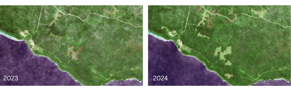
Fig. 2. Examples of GeoMAD data of the same area in 2023 (left) and 2024 (right).
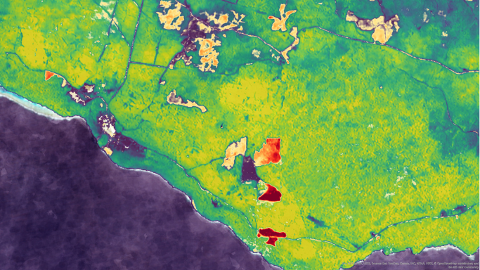
Fig. 3. Detected vegetation clearing between 2023 and 2024.
2. From Mapping to Monitoring
The most important contribution of this work is not simply vegetation height estimation. It is operational vegetation structure monitoring over time.
Because the dataset is produced consistently at quarterly intervals across five years, it becomes possible to monitor structural vegetation change rather than relying only on isolated snapshots.
This enables workflows such as:
- identifying deforestation trajectories
- monitoring regrowth and restoration
- observing cyclone and disturbance impacts
- comparing vegetation structure consistently over time
- supporting biomass and carbon estimation
- generating long-term vegetation condition baselines
Many widely used vegetation products measure greenness or vegetation presence. By contrast, the Geoneon workflow estimates mean vegetation height, producing a representation of vegetation structure rather than simply vegetation activity.
Operationally, this creates a more interpretable view of landscape change. A reduction in vegetation height can indicate clearing, degradation, or disturbance, even where residual greenness remains visible in spectral imagery.
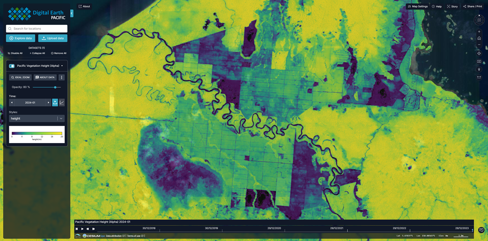
Fig. 4. Farmland and river systems in Papua New Guinea shown on the Digital Earth Pacific platform, illustrating vegetation structure changes.
The quarterly structure of the dataset also changes the monitoring workflow itself. Instead of observing vegetation change retrospectively through annual products, vegetation structure can now be tracked progressively through time across consecutive quarters.
The important shift is that vegetation structure monitoring no longer depends entirely on sparse airborne surveys or isolated local studies. By combining machine learning with routinely refreshed Sentinel-2 imagery, the workflow makes it possible to observe structural vegetation change consistently across very large regions and through time.
3. How Vegetation Structure Can Be Inferred from Imagery
One of the central insights in the project is that vegetation structure can be inferred from image texture and spectral behaviour, even where direct vegetation height measurements are sparse or unavailable.
In practical terms, vegetation height is strongly associated with how vegetation appears spatially within imagery. Dense forest canopies, fragmented vegetation, grasslands, and cleared land all exhibit different spatial texture and spectral behaviour. The workflow uses these patterns to infer mean vegetation height at 10 metre resolution.
Importantly, the work showed that preserving vegetation structure within the imagery itself is critical for successful vegetation height estimation.
The project compared two imagery approaches:
- GeoMAD composites
- Copernicus Quarterly Cloudless Mosaics
GeoMAD composites prioritise spectral consistency and robustness across long time windows, but the compositing process can smooth spatial texture and reduce fine vegetation detail.
The Cloudless Mosaics behaved differently. Instead of emphasising temporal smoothing, they preserved sharper vegetation structure, edges, and local texture. This proved important because the machine-learning workflow relied heavily on visible vegetation structure patterns within the imagery.
In practice, the Cloudless Mosaics generally produced more realistic vegetation height estimates and broader vegetation-height variation than GeoMAD imagery. This became one of the most important findings of the work: preserving spatial vegetation texture can matter more than maximising spectral smoothness when estimating vegetation structure from RGB imagery.
GeoMAD imagery examples
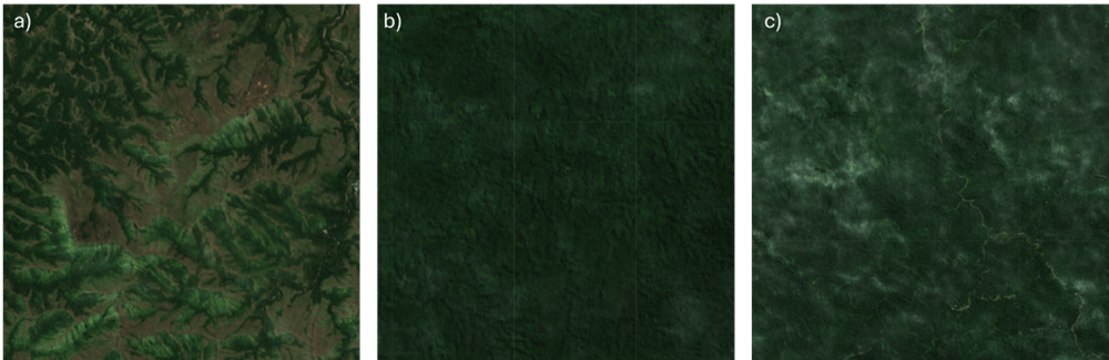
Fig. 5. Examples of GeoMAD data. a) Cloudless. b) Slightly cloudy. c) Very cloudy. GeoMAD composites improve spectral consistency across long time windows, but can smooth vegetation texture and reduce structural detail important for vegetation height inference.
Cloudless Mosaic imagery examples
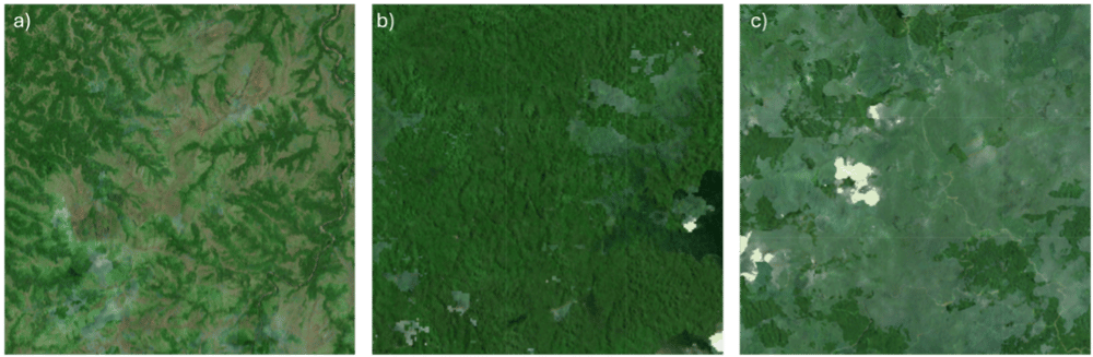
Fig. 6. Examples of Cloudless Mosaics data in the same locations as Figure 1. a) Cloudless. b) Slightly cloudy. c) Severe cloud cover. Quarterly Cloudless Mosaics preserve sharper vegetation structure and spatial texture, improving the visibility of canopy patterns used in vegetation height estimation.
GeoMAD vs Cloudless comparison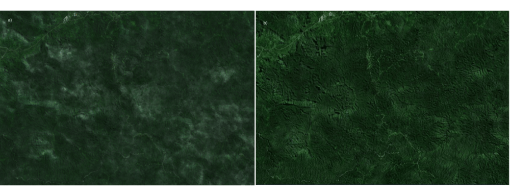
Fig. 7. Image of an area in Fiji in 2023. a) GeoMAD. b) Cloudless mosaics. This comparison illustrates how GeoMAD compositing can smooth vegetation structure relative to Cloudless Mosaics.
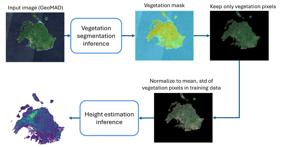
Fig. 8. Full multi-step vegetation height inference pipeline using vegetation segmentation mask for ocean exclusion.
Figure 4 shows how the height maps are derived from GeoMAD data. The input data (color, brightness and contrast) are prepared to ensure they are similar to the height model training data. A segmentation model produced the vegetation mask that helps to extract all the vegetation pixels from the input image. Non-vegetation pixels are set to no-data in the vegetation-extracted input. Consequently, the final height map would present non-vegetation pixels as no-data.
4. Building the Monitoring Workflow
4.1 Creating Training Data at Regional Scale
One of the main technical challenges was the lack of large-scale vegetation height labels across the Pacific. To address this, Geoneon developed a multi-stage training workflow.
The process began by generating vegetation height labels from LiDAR-derived Digital Surface Models (DSM) and Digital Terrain Models (DTM). These labels were used to train an initial 1 metre vegetation height model using high-resolution aerial imagery.
That 1 metre model was then applied across many additional high-resolution image tiles to generate pseudo-labelled vegetation height data. These pseudo-labels were subsequently aggregated down to 10 metre resolution and used to train the final large-area vegetation height model.
This effectively bootstrapped a large vegetation height training dataset from relatively sparse measured data.
Mathematically, the final product estimates mean above-ground vegetation height within each 10 metre pixel, meaning the dataset represents average vegetation structure rather than maximum canopy height.
This distinction matters operationally because it produces a more stable and comparable representation of landscape-scale vegetation condition suitable for long-term monitoring workflows.
Vegetation height model development workflow
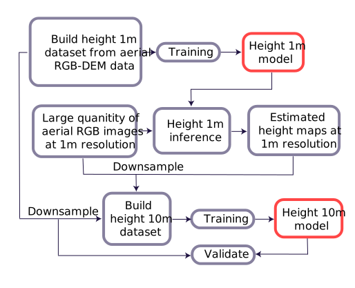
Fig. 9. Vegetation height model development workflow showing LiDAR-derived training labels, pseudo-labelling, aggregation to 10 metre resolution, and final large-area vegetation height model training.
4.2 Building a Time-Series Workflow
The most important operational design choice was building the workflow as a quarterly time-series dataset rather than a single-date mapping product. This changes the role of the product substantially.
Instead of simply generating a vegetation height layer for one point in time, the workflow supports repeated structural vegetation observation across multiple years.
The quarterly products spanning 2020–2025 make it possible to:
- monitor progressive vegetation clearing
- observe vegetation recovery
- detect disturbance trajectories
- compare structural vegetation change consistently through time
This transforms the workflow from a mapping exercise into an operational monitoring system.
5. What we found
5.1 Vegetation structure behaved consistently across landscapes
Across the Pacific case studies, the vegetation height products generally behaved as expected.
Dense forests appeared as high vegetation areas, grasslands and cleared areas appeared lower, and roads or non-vegetated surfaces appeared close to zero height or as masked areas. Stable vegetation areas also tended to remain consistent over time.
This is an important operational outcome because the usefulness of a vegetation structure product depends on whether structural patterns remain physically interpretable across many different landscapes and monitoring periods.
The workflow showed encouraging consistency across outputs generated for Fiji and the Solomon Islands, with no major systematic flaws observed across wider regional results.
5.2 Structural Canopy Loss Became Clearly Visible
One of the strongest outcomes of the project was the visibility of deforestation and degradation within the vegetation height time series.
In the Solomon Islands examples, forest clearing appeared not only as a colour change in RGB imagery, but as a clear structural collapse in inferred vegetation height. Dense forest areas transitioned into substantially lower vegetation-height classes following clearing activity.
This is an important distinction. The workflow does not simply monitor vegetation greenness. It monitors vegetation structure. As a result, change becomes visible in terms of structural canopy loss rather than only spectral variation.
This creates a more interpretable representation of landscape change, particularly across heterogeneous forest systems where greenness alone may not clearly distinguish degradation from intact vegetation.
Vegetation height deforestation trajectory examples
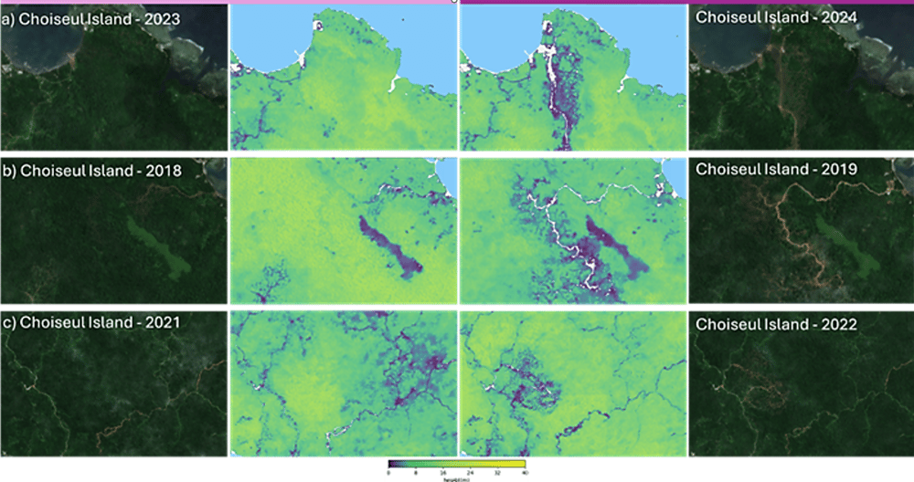
Fig. 10. Vegetation height monitoring outputs showing structural canopy loss associated with deforestation in the Solomon Islands. Structural vegetation change becomes clearly visible through the quarterly height time series.
Several important patterns become visible in these examples.
First, the vegetation height estimation behaves consistently across different landscape types. Dense forests appear substantially higher than surrounding vegetation systems, grass-dominated areas remain low, and roads appear clearly as no-data within the height surfaces.
Second, severe clearing trajectories become highly visible within the vegetation structure outputs. In multiple examples, progressive canopy removal can be observed directly through reductions in inferred vegetation height, while surrounding unchanged forest areas remain comparatively stable where the image quality is good.
Third, the examples also highlight one of the workflow’s major limitations. In areas affected by cloud or haze contamination, vegetation height can become underestimated because the model was trained primarily on cloud-free imagery. This becomes particularly visible in parts of the Solomon Islands examples and reinforces the importance of confidence layers and observation-density tracking within the broader monitoring workflow.
5.3 Quarterly Monitoring Revealed Progressive Change
The quarterly structure of the dataset enabled another important capability: progressive monitoring of vegetation structure change over time.
Instead of observing disturbance only retrospectively through annual products, vegetation structure could be tracked incrementally across consecutive quarters.
This made it possible to observe:
- progressive clearing
- gradual degradation
- disturbance recovery
- evolving land-use change
The shorter temporal windows also improved visual interpretability by reducing the smoothing effects associated with long-period image compositing.
Quarterly vegetation change progression
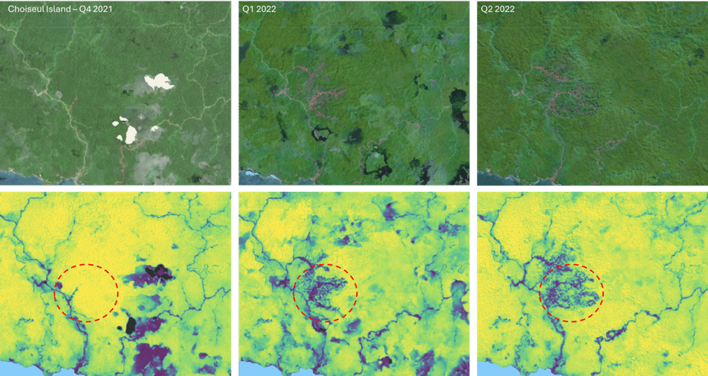
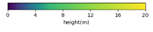
Fig. 11. Quarterly vegetation height monitoring outputs showing progressive vegetation change over time. Consecutive quarterly products improve the visibility of evolving disturbance and recovery trajectories.
6. Validation and Limitations
6.1 What the Vegetation Height Product Represents
The product estimates mean above-ground vegetation height within each 10 metre pixel. It does not attempt to estimate maximum canopy height or replace high-resolution LiDAR measurements directly.
This distinction matters because the product is designed primarily for regional vegetation structure monitoring and change detection rather than fine-scale forest inventory applications.
GEDI validation work and comparison exercises suggest that the workflow produces realistic relative vegetation structure patterns, while also highlighting expected uncertainty associated with cloud contamination and complex vegetation environments.
The outputs should therefore be interpreted as planning-grade vegetation structure layers suitable for monitoring and change analysis workflows.
6.2 Cloud Cover Remains the Main Limitation
Cloud cover remains the biggest limitation in the workflow.
Because the models were trained primarily on cloud-free imagery, clouds, mist, and cloud shadows tend to reduce inferred vegetation height values. This can introduce systematic underestimation in affected areas.
The issue affects both GeoMAD and Cloudless Mosaic workflows differently:
- GeoMAD reduces cloud artefacts through temporal smoothing
- Cloudless Mosaics preserve vegetation detail more effectively but remain more sensitive to residual cloud contamination
To help address this operationally, the workflow introduced confidence layers based on local observation density during mosaicking. Areas with fewer valid observations can therefore be interpreted more cautiously within downstream monitoring workflows.
Cloud cover deteriorates the height estimation
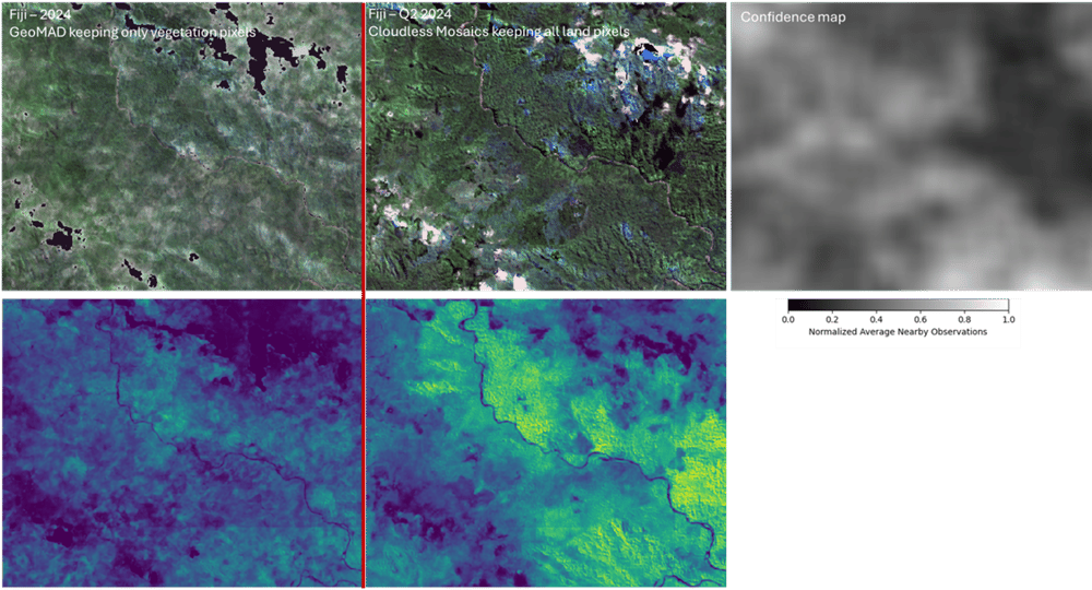
Fig. 12. Left: GeoMAD results - Severe cloud cover is classified as non-vegetation, hence appearing as no-data (black) on the vegetation height map. Mild cloud cover is classified as vegetation, but the height is greatly underestimated.
Right: Cloudless Mosaics results- The clouds in the image mean they passed through the cloud filter algorithm to end up here. These cloudy areas have low confidence in the confidence map as well as low height estimated.
6.3 Coastlines and Land Masks Matter More Than Expected
The project also found that land masking becomes operationally important across Pacific environments because ocean pixels can distort RGB normalisation and influence model behaviour.
Several masking approaches were evaluated, including:
- vegetation masks
- OpenStreetMap land polygons
- GADM land polygons
OpenStreetMap polygons ultimately produced the best operational balance because they provided finer coastline detail while preventing vegetation height estimation over open ocean areas.
7. Designed for Repeat Monitoring at Regional Scale
A major reason this workflow is useful in practice is that it is designed around repeatable production and monitoring continuity.
The system depends primarily on routinely available Sentinel-2 imagery and scalable machine-learning inference rather than bespoke local airborne campaigns.
Operationally, the workflow provides:
- quarterly monitoring from 2020–2025
- consistent 10 metre vegetation structure outputs
- regional-scale deployment capability
- refreshable production workflows
- comparable outputs across years and jurisdictions
This means the workflow is not simply a one-off vegetation mapping exercise. It is a vegetation monitoring pipeline designed to support repeated structural observation across large geographic regions.
The outputs are designed to support operational monitoring and reporting workflows across the Pacific, including planning, restoration, biomass estimation, and climate reporting applications.
8. Toward Long-Term Vegetation Structure Monitoring
The project also identified several important future directions.
The most immediate is improved cloud filtering and confidence estimation. Because cloud contamination remains one of the dominant sources of uncertainty, more advanced cloud handling is likely to improve temporal consistency and vegetation height accuracy further.
Additional future directions include:
- improved coastal and mangrove masking
- enhanced temporal consistency between quarters
- expanded validation datasets
- integration with biomass estimation workflows
- improved disturbance and regrowth detection
More broadly, the work demonstrates that repeat vegetation structure monitoring is now possible across very large and geographically fragmented regions using routinely available satellite imagery.
The significance of the project is not simply that vegetation height can be estimated from Sentinel-2 imagery. It is that quarterly vegetation structure monitoring can now support long-term ecosystem observation, deforestation tracking, restoration monitoring, and climate reporting workflows across the Pacific at regional scale.
9. Acknowledgements
This work was delivered by Geoneon and D4DInsights in partnership with the Pacific Community (SPC) through its Digital Earth Pacific programme, which commissioned and guided the development to address regional priorities. The Digital Earth Pacific and D4DInsights contributors, included Andiswa Mlisa, Sachindra Singh, Aditya Agrawal, Brian Killough, Alex Leith, and Jesse Anderson.